Introduction

Self-avoiding walks

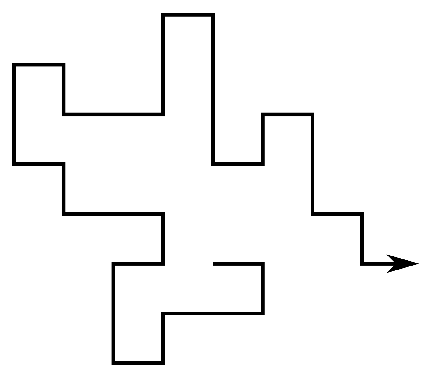
A self-avoiding walk (SAW) $\omega$ is a sequence of lattice vertices $(\omega_0, \omega_1, \dots, \omega_n)$ such that $\omega_i \neq \omega_j$ for $i\neq j$, and $\omega_i,\omega_{i+1}$ are adjacent on the lattice for each $i=0,\dots,n-1$. We say $\omega$ has size $|\omega| = n$.

Since the lattice is vertex-transitive, if one SAW is a translation of another we consider them to be the same. Equivalently assume $\omega_0 = 0$.

For a given lattice take $c_n$ to be the number of SAWs of size $n$. Then e.g. on the square lattice \[ (c_n)_{n\geq0} = (1, 4, 12, 36, 100, 284, 780, \dots) \]

Self-avoiding polygons

A self-avoiding polygon (SAP) $\pi$ is a sequence of lattice vertices $(\pi_1, \pi_1, \dots, \pi_{n})$ such that $\pi_i \neq \pi_j$ for $i\neq j$, and $\pi_i,\pi_{i+1}$ are adjacent on the lattice, and so too are $\pi_1,\pi_n$. The size of $\pi$ is $n$.

Equivalently a SAP is a SAW which ends adjacent to its initial vertex.

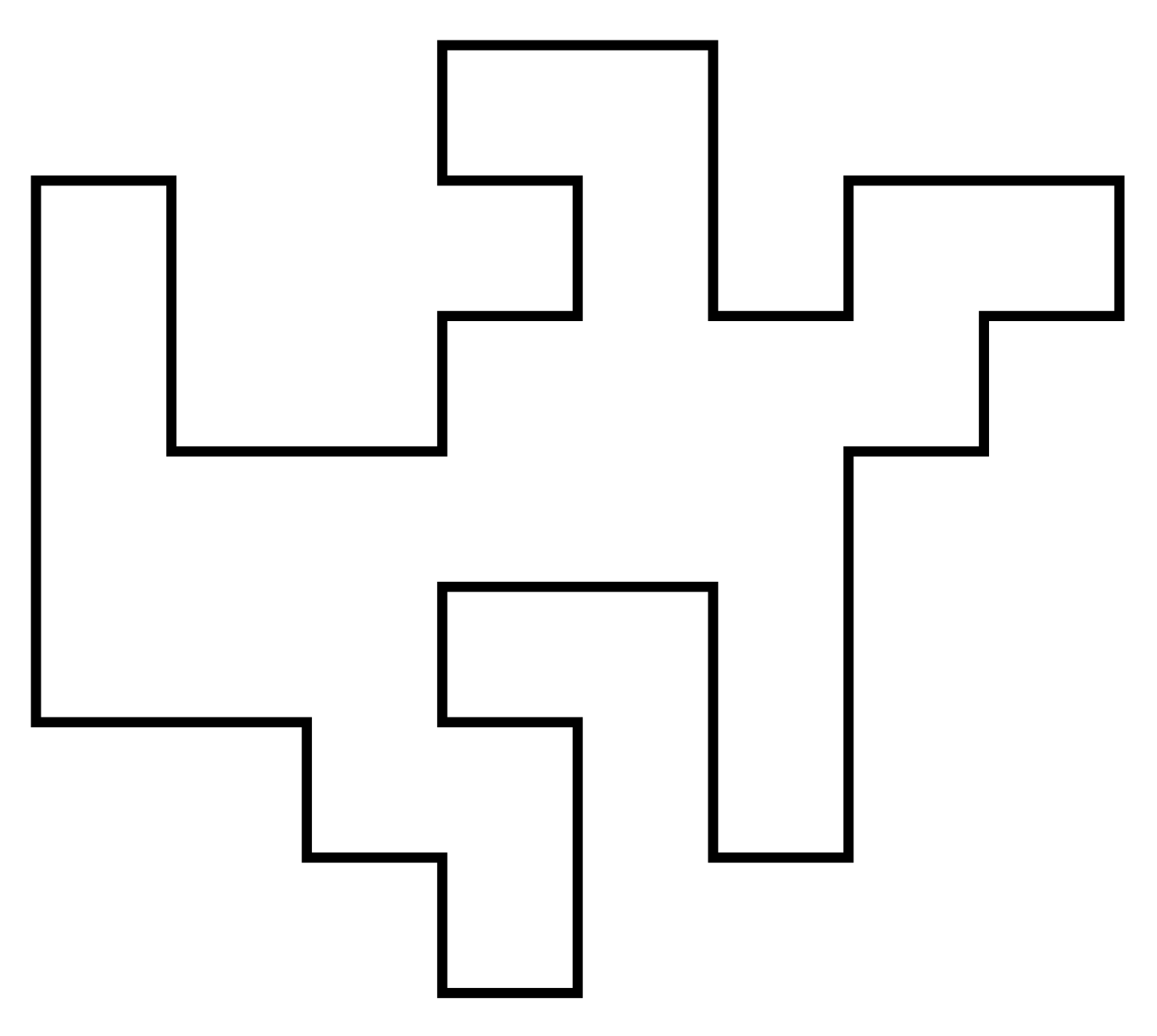
For our purposes two SAPs are the same if they are translates of one another. So there are $2n$ SAWs (of length $n-1$) corresponding to each SAP of size $n$. Let $p_n$ be the number of size-$n$ SAPs. Then e.g. on the square lattice \[ (p_n)_{n\geq4} = (1,0,2,0,7,0,28,0,124,\dots) \] (On the triangular and fcc lattices SAPs can have odd size.)

Thetas

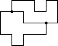
SAPS have all vertices of degree 2 while SAWs have two vertices of degree 1. Here we introduce vertices of degree 3: thetas (two vertices of degree 3).

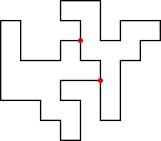Again counted up to translation. On the square lattice \begin{align*} (\theta_n)_{n \geq 7} &= (2, 0, 12, 6, 62, 60, 338, 430, 1966, \dots) \end{align*}

Lattices

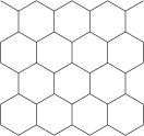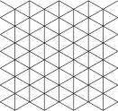
On the square and cubic lattices, the three "arms" of a theta must have the same parity $\rightarrow$ strong parity effects. Not a problem on the triangular or fcc lattices.

Motivation

The size of knots

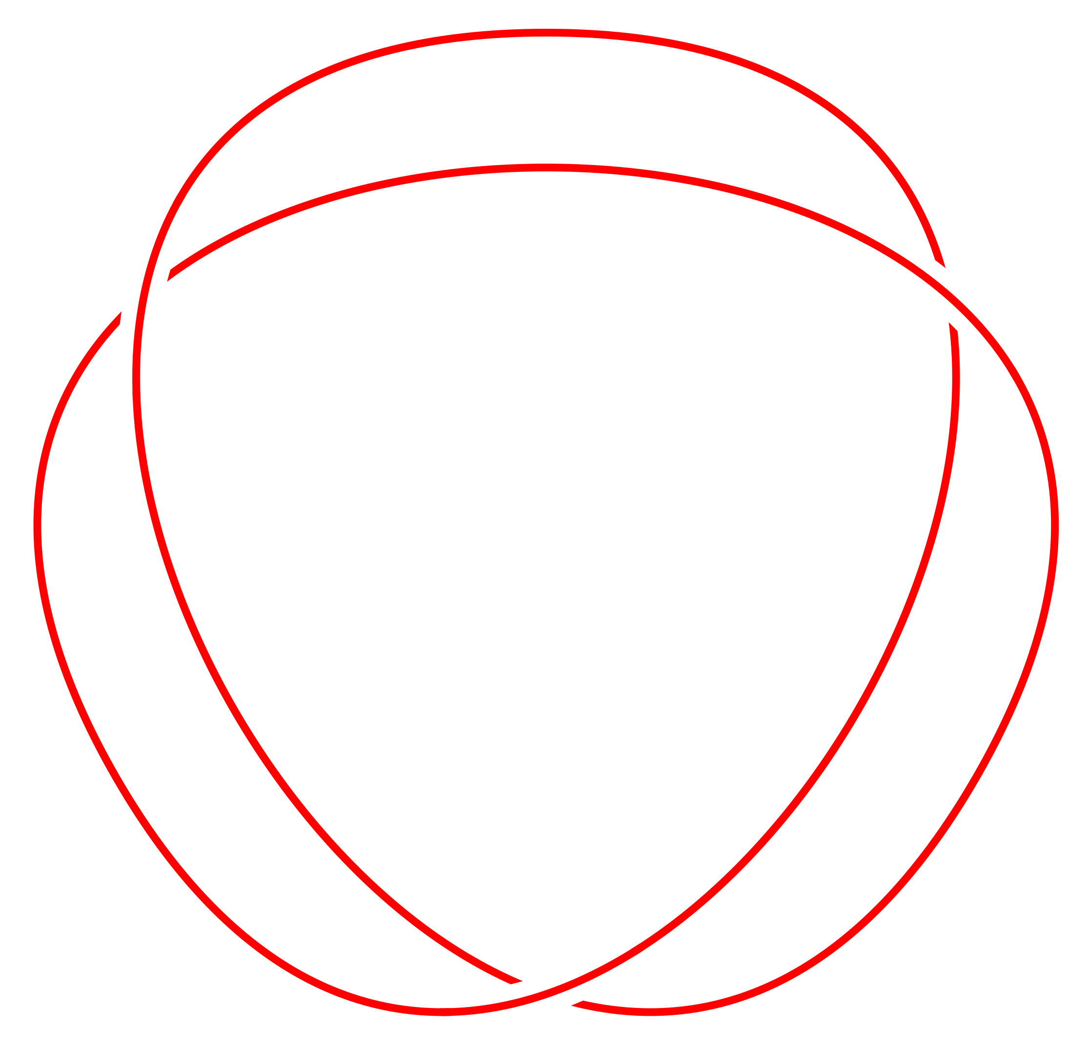
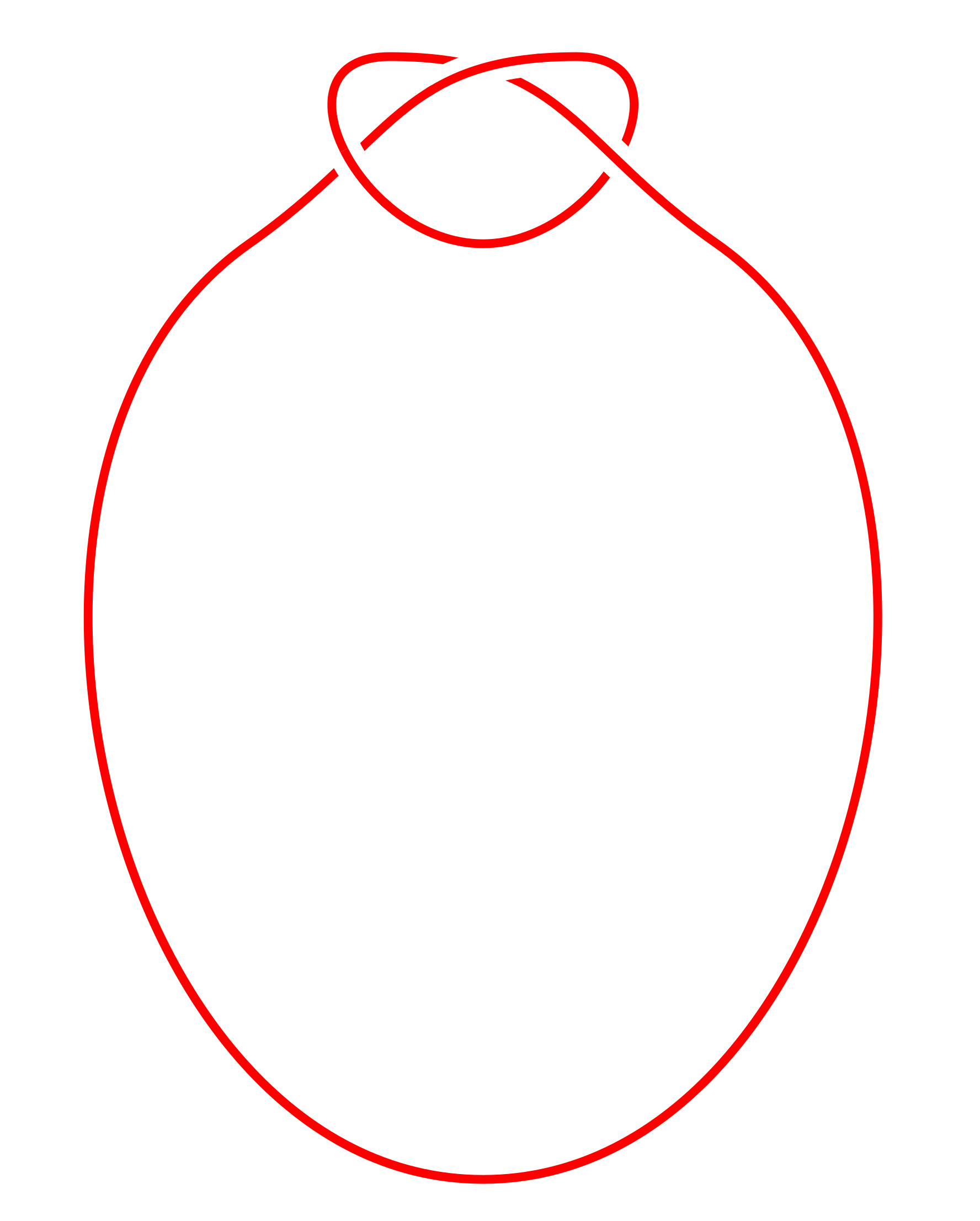
Knots are very likely because small "knotted parts" can be inserted into a polygon and force it to be knotted. But in turn the "knotted part" of a typical large knotted polygon is relatively small.

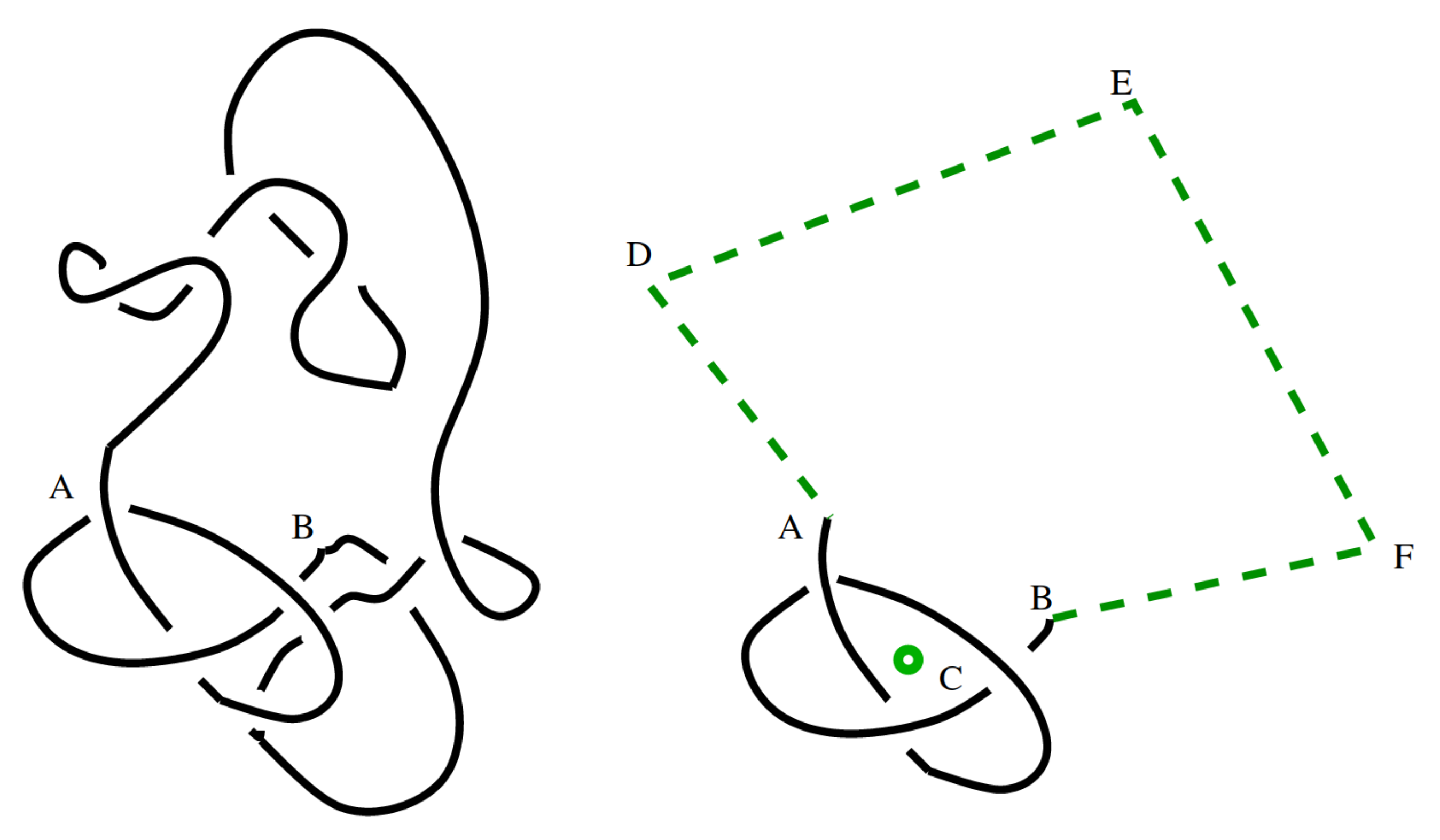
Different ways to estimate the "size" of the knotted part. Marcone et al (J. Phys. A 2005) use two different methods:

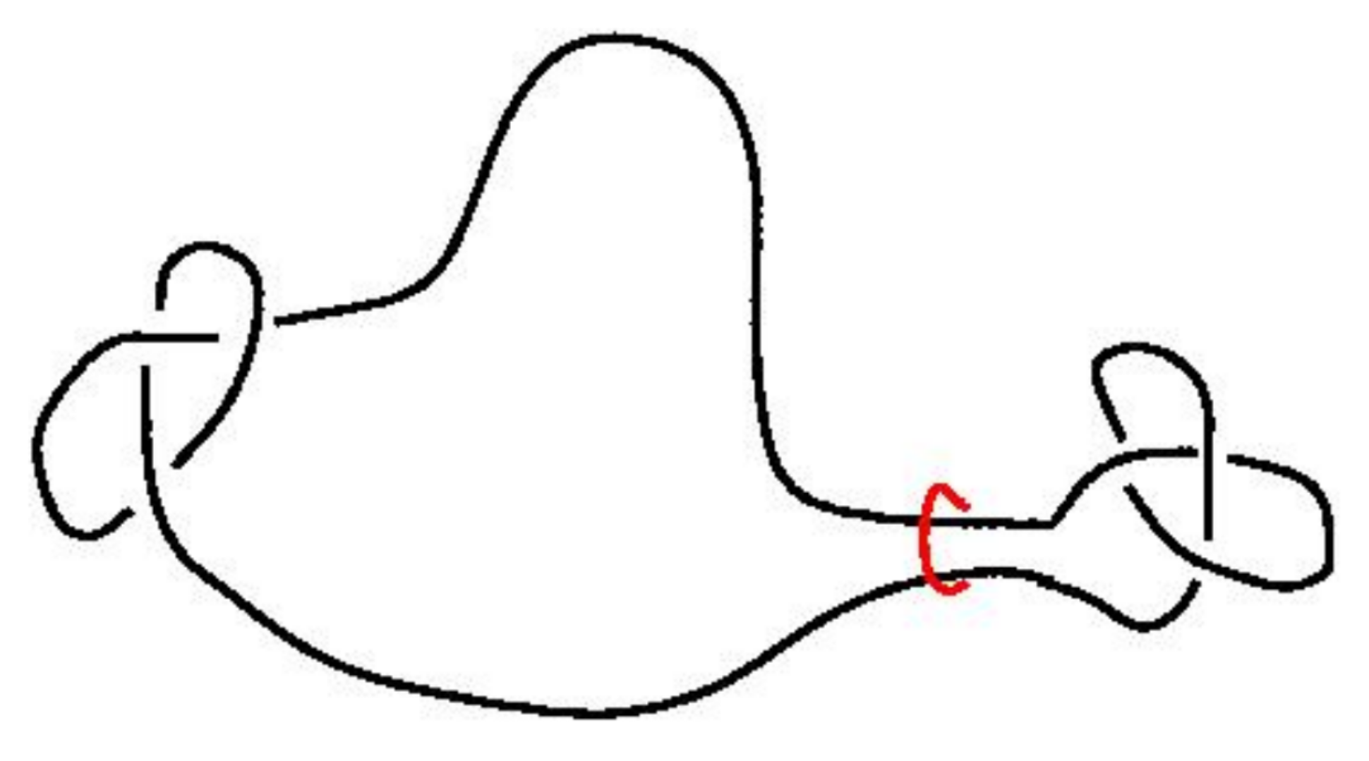Both methods lead to an estimate of the knotted part of an $n$-edge prime knot occupying $\approx n^{0.75}$ edges on average.

Knots vs. thetas

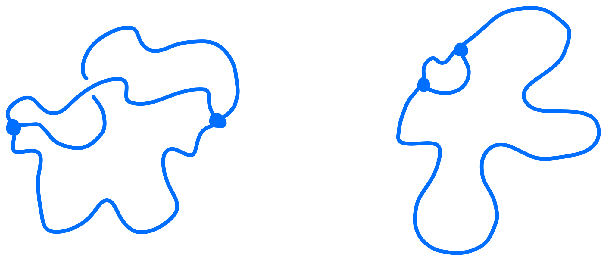
Question: How do the different parts of a typical theta scale in size? Most likely two arms are small and one big:

R-loops

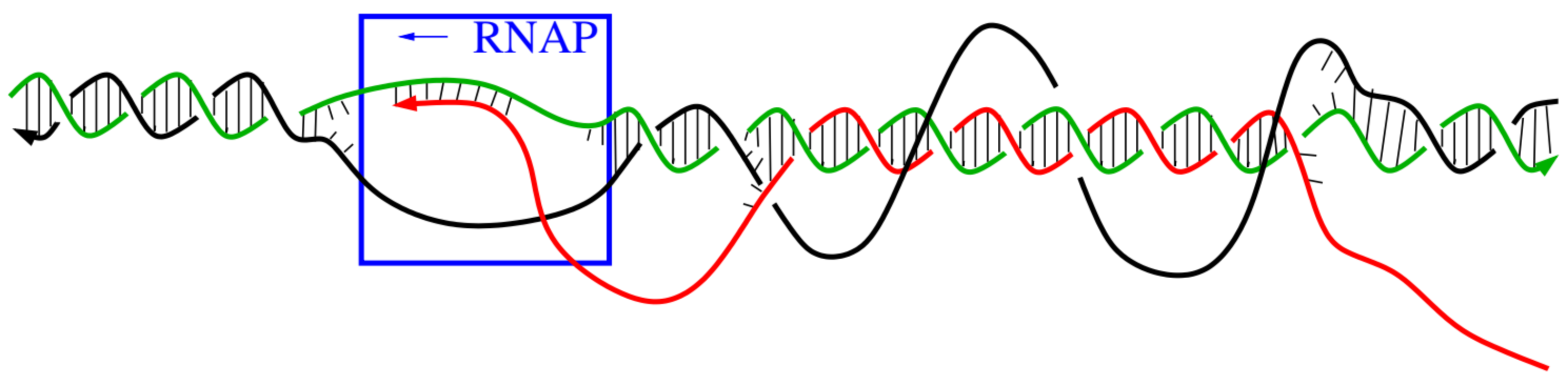
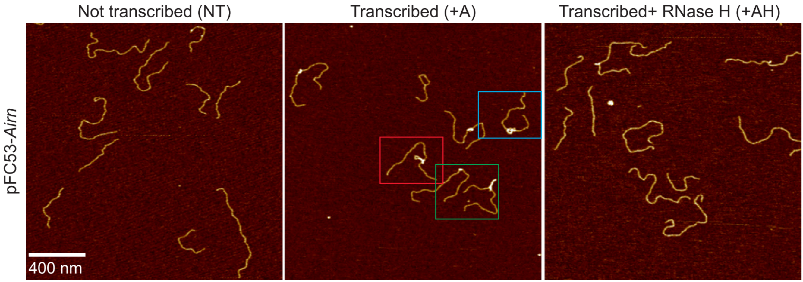
During DNA transcription, single-stranded RNA can fuse with double-stranded RNA to form R-loops:

Jonoska et al, Using Mathematics to Understand Biological Complexity 2021

Carrasco-Salas et al, Nucleic Acids Res. 2019

The presence of R-loops can affect repair, eg. in human cells.

R-loops

Topologically the DNA:RNA hybrid is a graph with two vertices of degree 3 or 4:

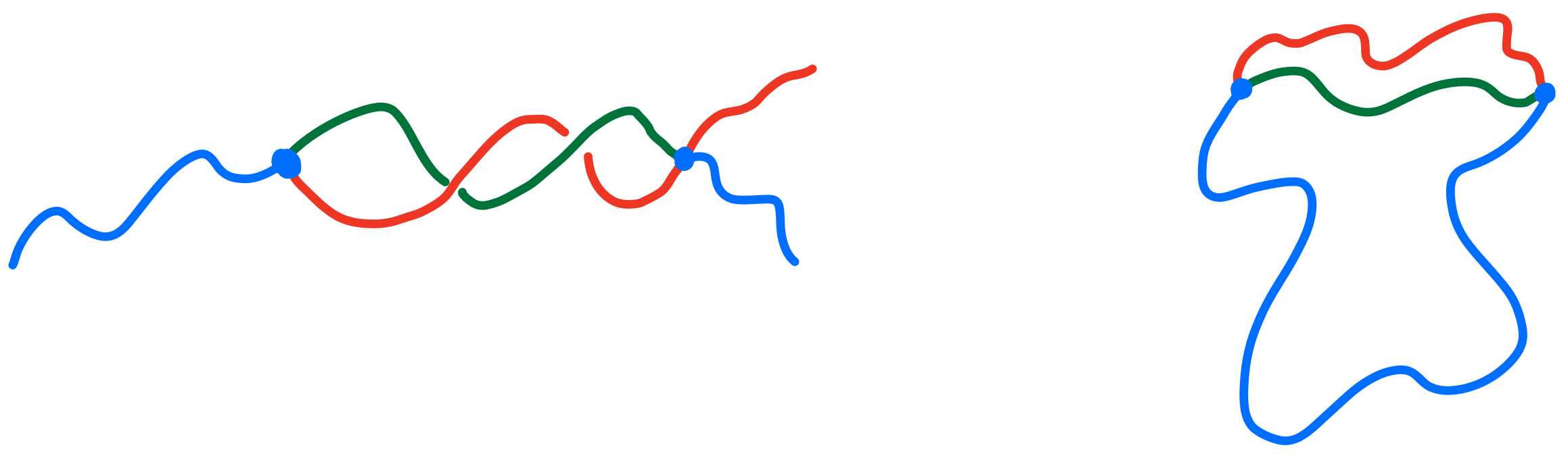
Different parts are single- or double-stranded so may have different stiffness etc.

Knotted theta-graphs

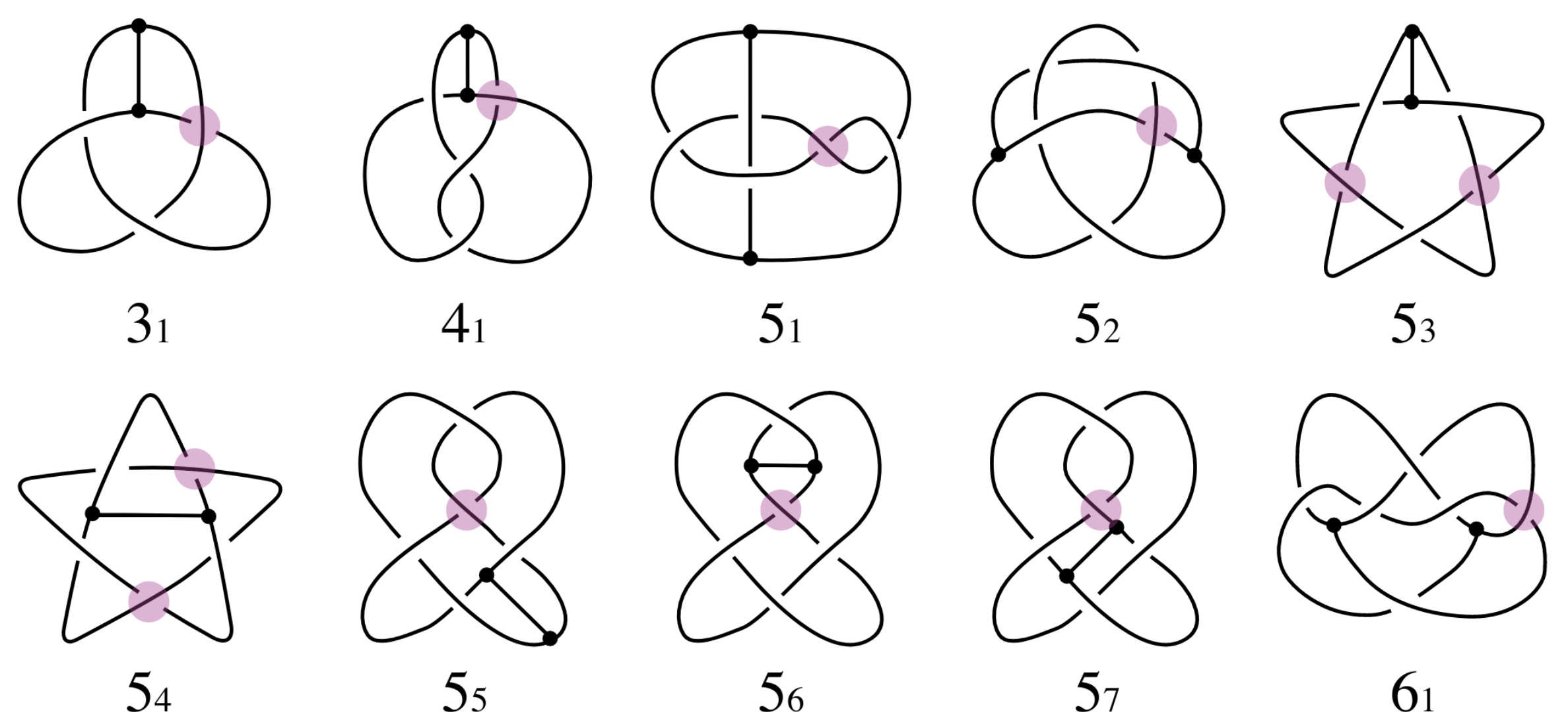
Thetas can also have non-trivial topology -- open questions about minimum number of edges required, etc.

Buck & O'Donnol 2018

Monte Carlo methods

BFACF algorithm

The BFACF algorithm (Berg & Foester 1981, Aragão de Carvalho, Caracciolo & Fröhlich 1983 and 1983) is a method for sampling SAWs and SAPs which preserves topology.

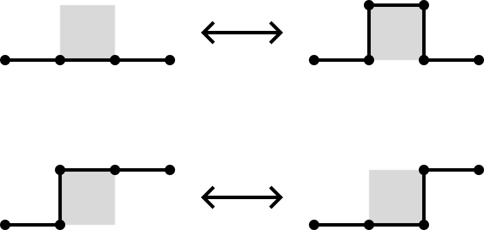
For 2D SAPs it is ergodic while in 3D the ergodicity classes are the knot types. For SAWs the ergodicity classes are walks between two fixed endpoints.

Also works on the triangular lattice.

BFACF algorithm

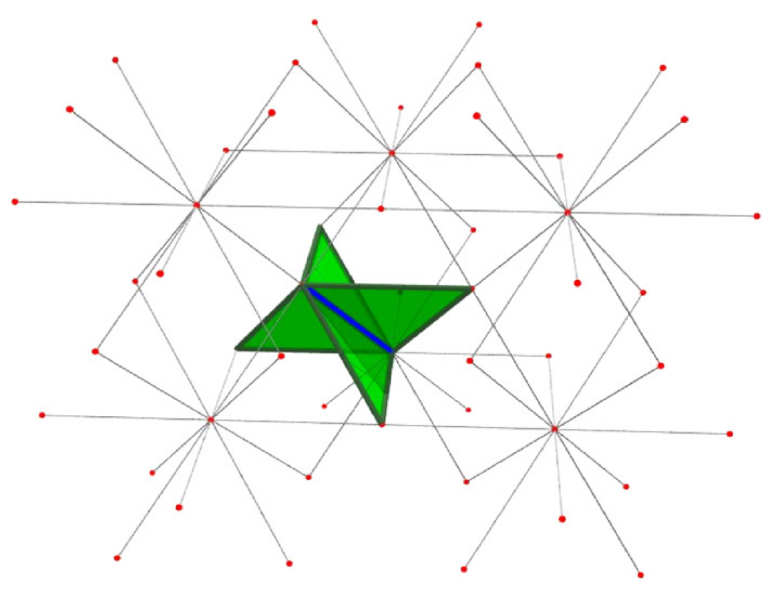
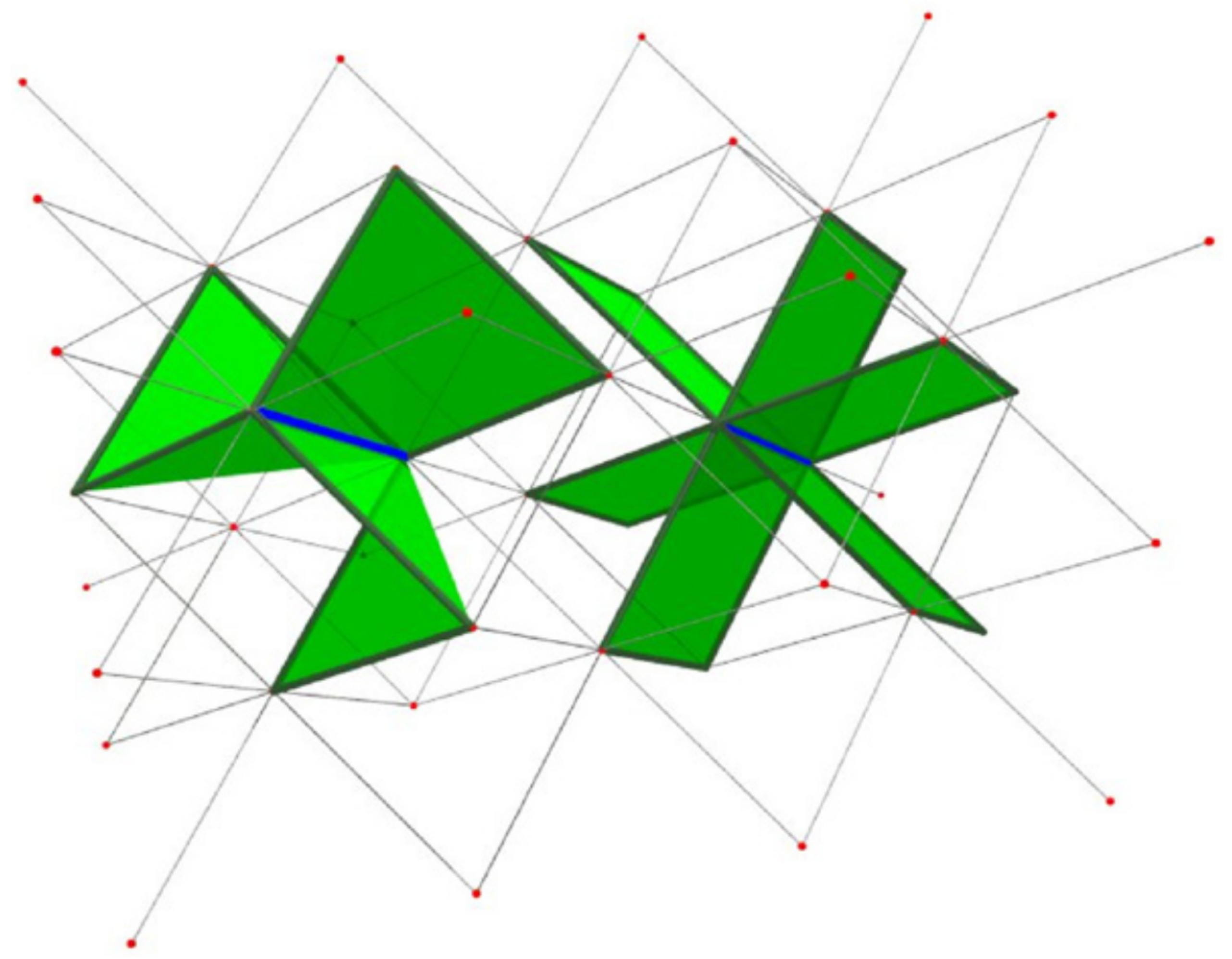
For the fcc and bcc lattices, Janse van Rensburg and Rechnitzer (2011) found a set of moves which also give the knot types as the ergodicity classes.

BFACF for branched structures

The above BFACF moves can shift vertices of degree 2 and leave vertices of degree 1 fixed.

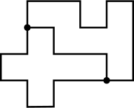
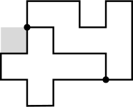
To accommodate vertices of degree 3, Tamaki (2018) found a new set of moves on the square/cubic lattices which can realise any ambient isotopic transformation:

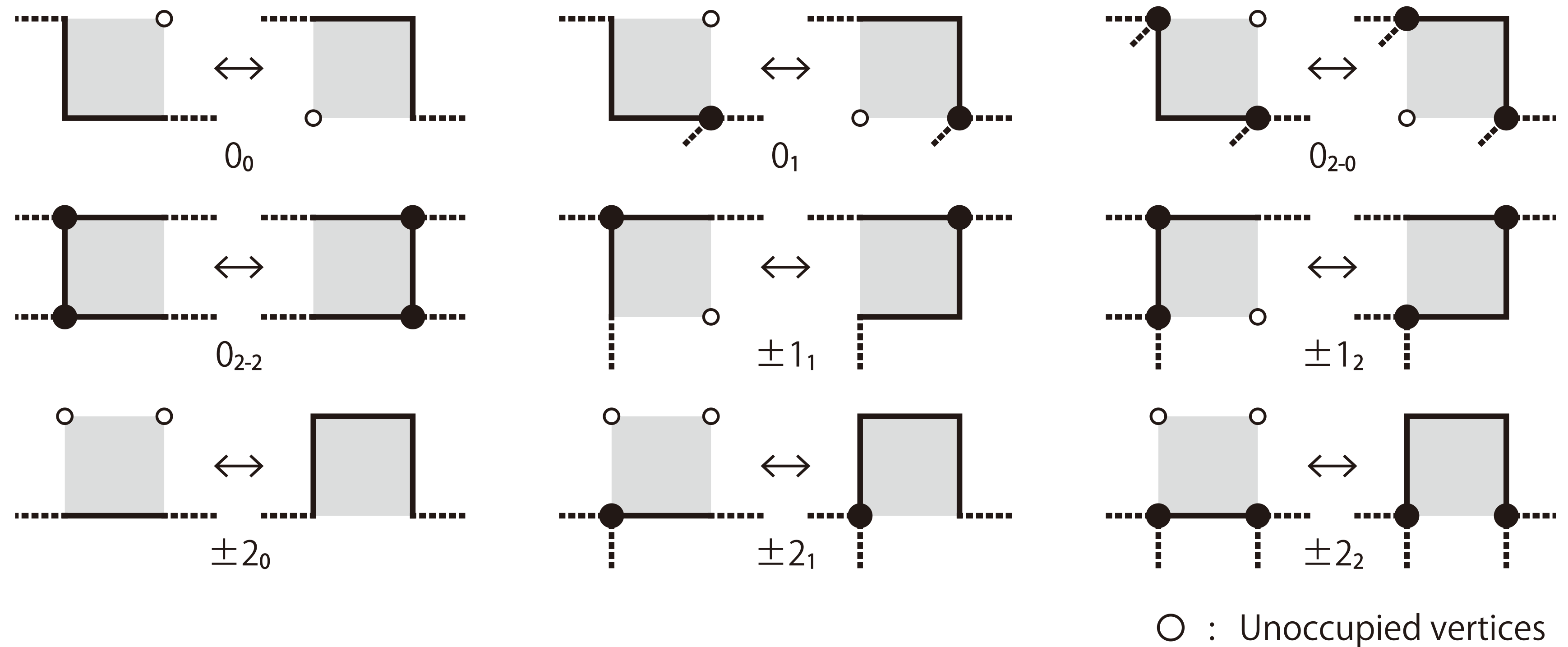
Note that the degree 3 vertices can move around.

BFACF for branched stuctures

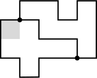
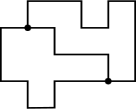
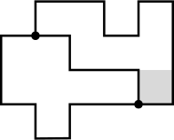
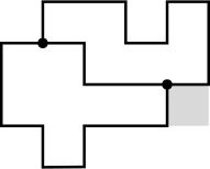
BFACF for branched structures

Simpler on the triangular lattice:

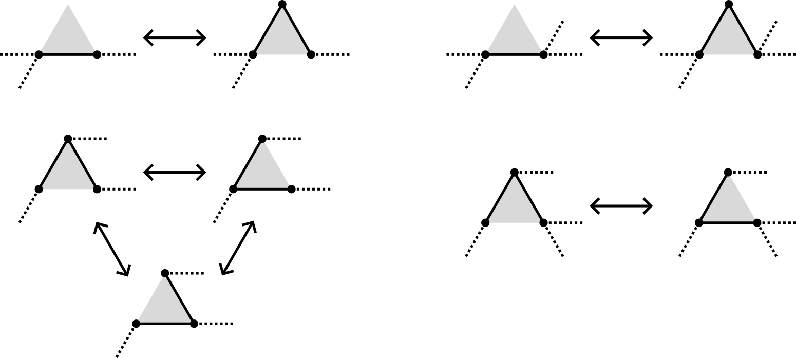
Same moves on the fcc lattice since the faces are still triangles.

Wang-Landau method

We combine the BFACF moves with the Wang-Landau method (2001) to estimate the number $a_n$ of configurations of size $n$.

Start with $f=1$ and arrays $G$ and $H$ both all $0$.

1. For a given configuration $\gamma$, pick a random edge and a random adjacent plaquette. If there is a valid BFACF move (changing $\gamma$ to $\gamma'$), accept with Metropolis probability \[ \mathbb{P}(\gamma \to \gamma') = \min\left\{1, \exp(G(|\gamma|) - G(|\gamma'|))\frac{w(\gamma'\to\gamma)}{w(\gamma\to\gamma')}\right\},\] else stay in state $\gamma$. Here $w(a\to b)$ is the probability that a randomly chosen move on state $a$ will change it to state $b$.
2. Now in state $\gamma''$ (either $\gamma$ or $\gamma'$), increment $G(|\gamma''|)$ by $f$ and $H(|\gamma''|)$ by 1.
3. If $H$ is sufficiently flat, decrease $f$ (e.g. $f \mapsto f/2$), reset $H=0$ and start again. Otherwise continue with the current value of $f$.
4. When $f$ reaches some small threshold, terminate.

If $m$ is the size of the smallest configuration, set $g=G(m)$ and then for each $n$ set \[ A(n) = \exp(G(n) - g)\cdot a_m. \] Then $A(n) \approx a_n$.

Wang-Landau method

Easily generalises to measure more than just size -- e.g. we will estimate $\theta_{n,k}$, the number of thetas of size $n$ with shortest arm of size $k$.

Many other variations -- e.g. change how $f$ decreases, or tune $G$ and then use those values to estimate some other quantity.

Results: 2D

Test case: the number of polygons

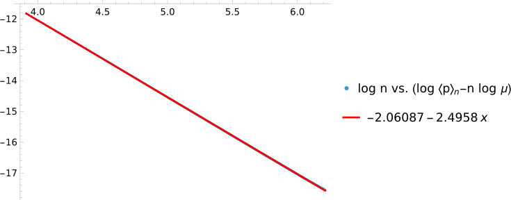
The number $p_n$ of SAPs on the lattice is $\sim \text{const.} n^g \mu^n$ where (Guttmann 2009) \[ g = \begin{cases} -5/2 & d=2 \\ -2.76279 & d=3 \end{cases} \] and $\mu$ is the connective constant of the lattice (Jensen 2004, Clisby 2022): \begin{align*} \mu_\text{tri} &= 4.150797226(26) \\ \mu_\text{fcc} &= 10.03705785(14) \end{align*}

Test case: the number of polygons

Estimating the exponent $g$ for the triangular lattice (10 independent runs, $N=500$):

The number of thetas

Expect $\theta_n \sim \text{const.}n^h \mu^n$ for the same $\mu$.

Estimating the exponent $h$ for the triangular lattice (10 independent runs, $N=500$):

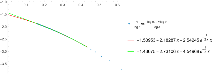
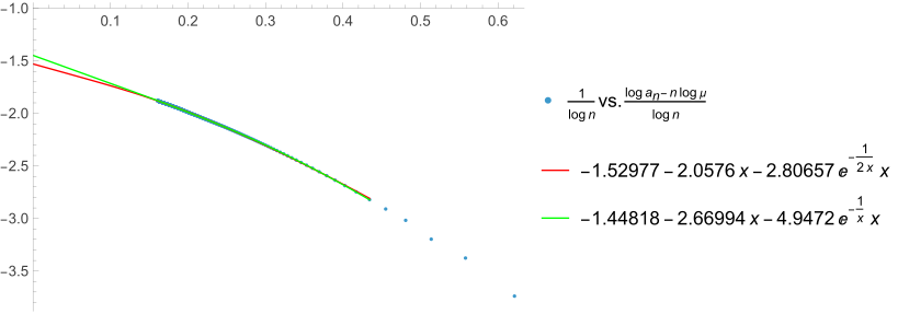
$h \approx g+1$ $\leftrightarrow$ $O(n)$ places to position a small loop within a big polygon.

The number of thetas

Estimating the exponent $h$ for the square lattice (10 independent runs, $N=500$):

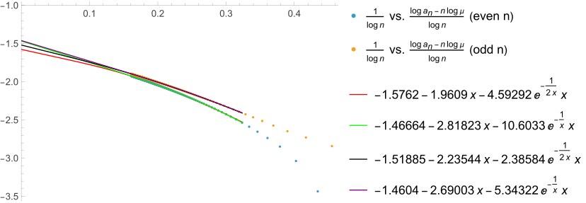
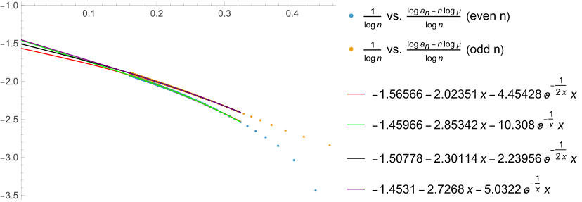
$h \approx g+1$ $\leftrightarrow$ $O(n)$ places to position a small loop within a big polygon.

Mean length of shortest theta arm

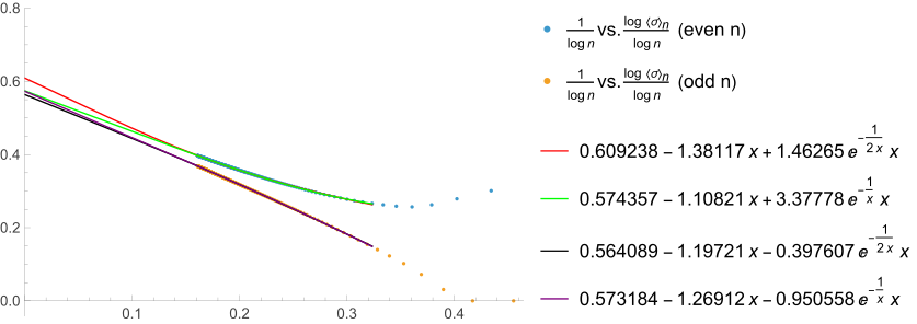
If $\sigma(\theta)$ is the length of the shortest arm then expect (?) $\langle \sigma \rangle_n \sim \text{const.}n^s$ for some $s$. Estimating $s$ for the triangular lattice (10 independent runs, $N=500$):

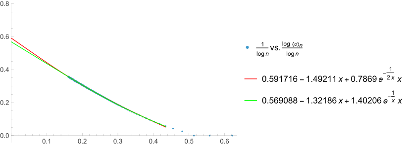
Mean length of shortest theta arm

Estimating $s$ for the square lattice (10 independent runs, $N=500$):

Mean length of second-shortest theta arm

Can also look at $\tau(\theta)$, the second-shortest (second-longest) arm. Triangular lattice (10 independent runs, $N=500$):

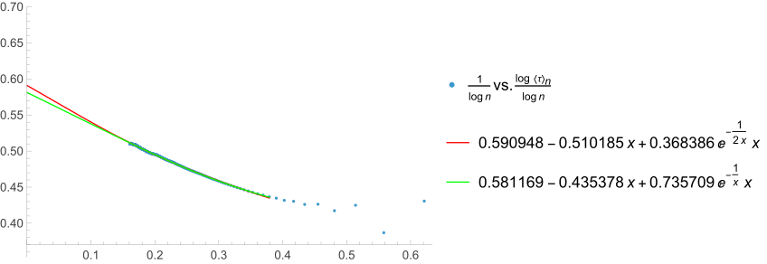
Likely the same exponent as for shortest arm.

Mean length of second-shortest theta arm

Square lattice (10 independent runs, $N=500$):

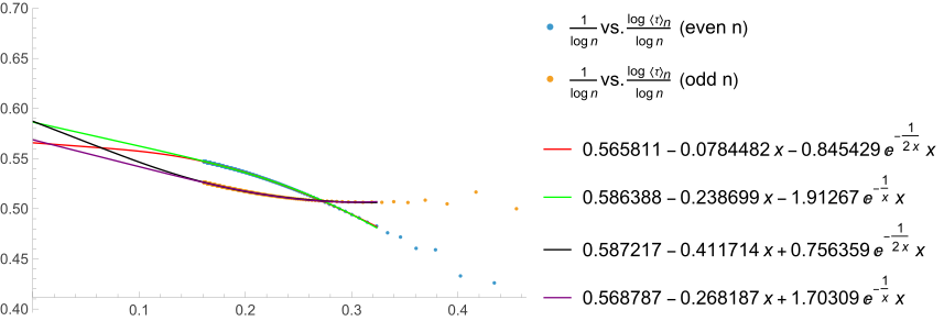
Likely the same exponent as for shortest arm.

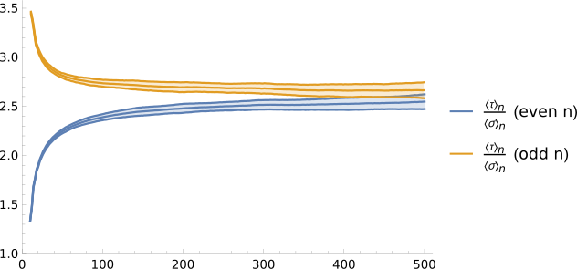
Ratio of second-shortest to shortest arm

Can also look at the ratio of the two. Expect it to approach a (lattice-independent?) constant. Triangular lattice (10 independent runs, $N=500$):

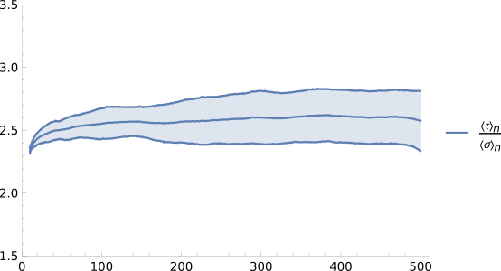
Ratio of second-shortest to shortest arm

Square lattice (10 independent runs, $N=500$):

Samples

$N=200$

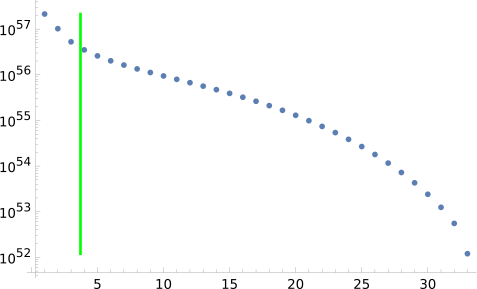
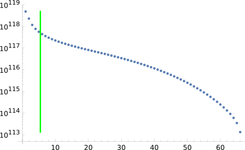
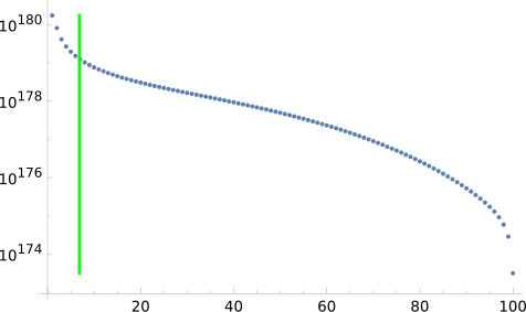
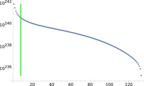
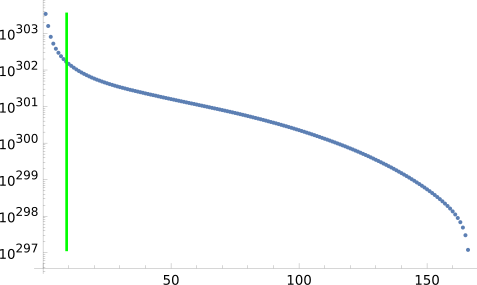
Distribution of $\sigma$

Distribution of the length of the shortest arm for triangular lattice (mean value indicated in green)

Results: 3D

The number of thetas

Estimating the exponent $h$ for the fcc lattice (10 independent runs, $N=400$):

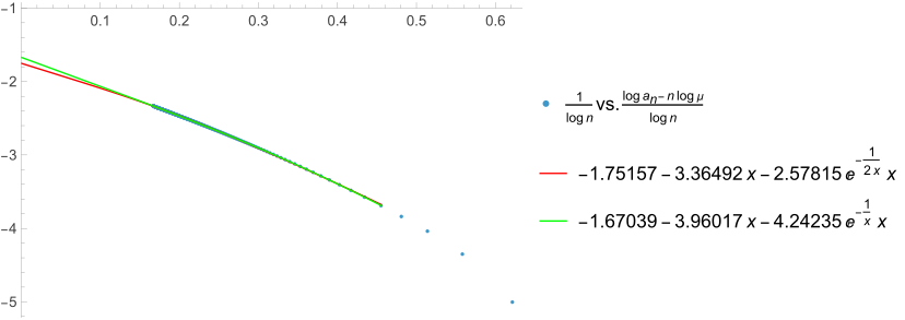
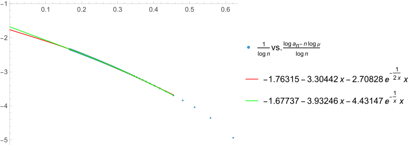
Recall that $g \approx -2.76279$ $\rightarrow$ again $h \approx g+1$.

Note that these thetas are unknotted so should really use $\mu_0$ but don't have an estimate for that.

The number of thetas

Estimating the exponent $h$ for the cubic lattice (10 independent runs, $N=400$):

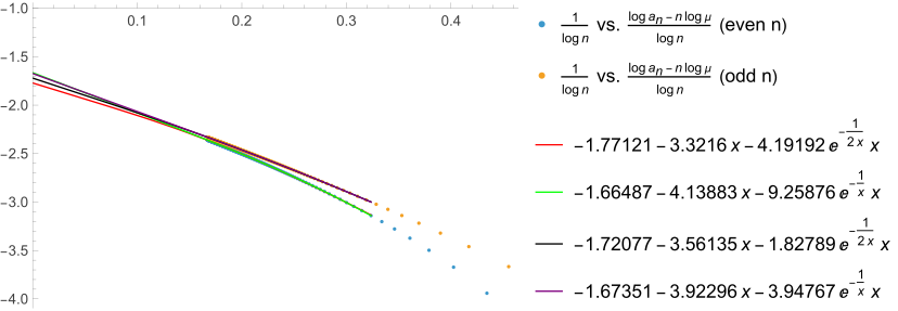
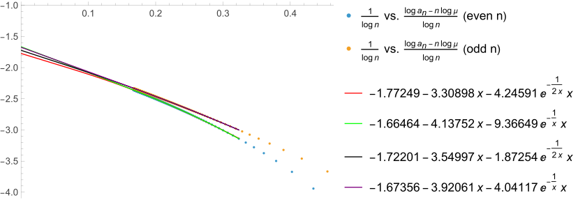
Again $h \approx g+1$.

Note that these thetas are unknotted so should really use $\mu_0$ but don't have a (good) estimate for that.

Mean length of shortest theta arm

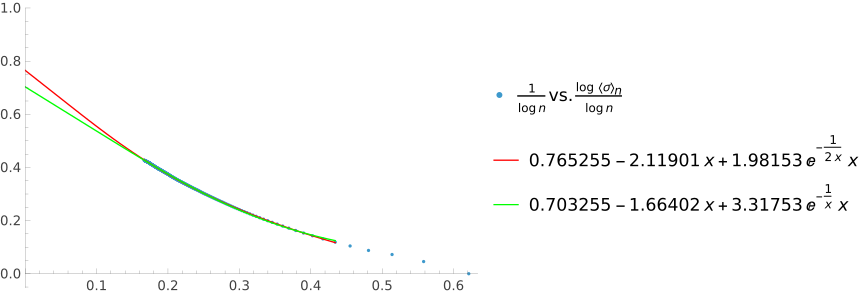
If $\sigma(\theta)$ is the length of the shortest arm then expect (?) $\langle \sigma \rangle_n \sim \text{const.}n^s$ for some $s$. Estimating $s$ for the FCC lattice (10 independent runs, $N=400$):

Mean length of shortest theta arm

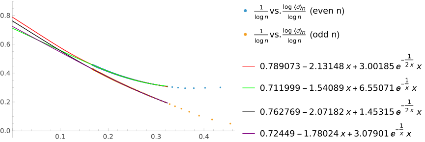
Estimating $s$ for the cubic lattice (10 independent runs, $N=400$):

Mean length of second-shortest theta arm

Can also look at $\tau(\theta)$, the second-shortest (second-longest) arm. FCC lattice (10 independent runs, $N=400$):

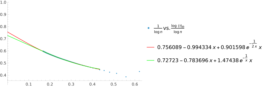
Likely the same exponent as for shortest arm.

Mean length of second-shortest theta arm

Cubic lattice (10 independent runs, $N=400$):

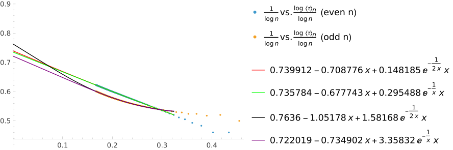
Likely the same exponent as for shortest arm.

Ratio of second-shortest to shortest arm

Can also look at the ratio of the two. Expect it to approach a (lattice-independent?) constant. FCC lattice (10 independent runs, $N=400$):

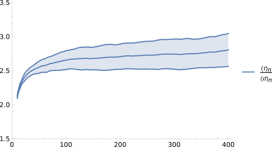
Ratio of second-shortest to shortest arm

Cubic lattice (10 independent runs, $N=400$):

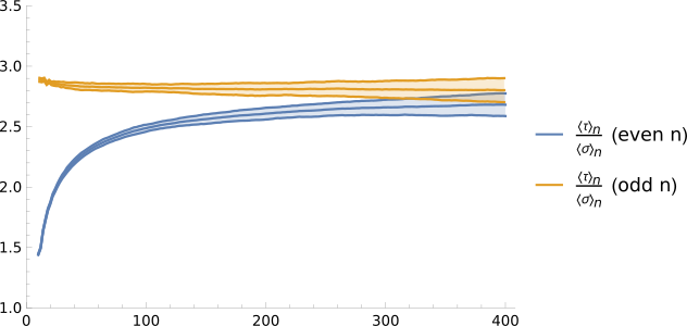
Distribution of $\sigma$

Distribution of the length of the shortest arm for FCC lattice (mean value indicated in green)

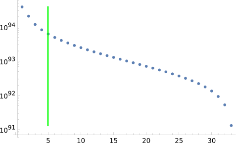
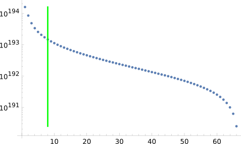
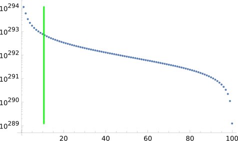
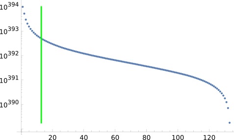
This contrasts with observed knot size distributions (linear chains) which seem to have a peak at fixed length and then power-law decay (Tubiana et al 2013).

Separation of tripoints

Mean squared distance between the two degree 3 vertices, fcc lattice, one single run (from last night!) to length 250:

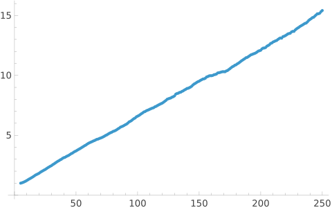
Scales like $n^\alpha$ with $\alpha \approx 1$

Compare this exponent with the "expected" value $\sigma\times2\nu \approx 0.88$. Tripoints seem to be "pushed apart". Similar behaviour in 2D.

Samples

$N=120$

Ongoing & future work

• Other shapes? (e.g. tadpoles, combs)
• Thetas with all three arms of equal length
• How do knots affect things?
• Minimum sizes of prime theta knots
• Introduce weights to model R-loops